Basel Committee’s Adjustments to the IRRBB Standard

---

On July 16, 2024, the Basel Committee on Banking Supervision (BCBS) announced targeted adjustments to the Interest Rate Risk in the Banking Book (IRRBB) standard. These updates, which stemmed from a consultative process initiated in December 2023, are critical for banks as they significantly impact how interest rate risks are measured and managed within banking books. This comprehensive analysis delves into the changes, their implications, and the next steps for banks.

---

Source

[1]

Reporting Standards: EBA on Banking Interest Rates

The EBA’s new ITS bring transformative changes to EU banking. Enhancing IRRBB assessment, transparency, and risk management. Balanced, proportional approach sets a precedent. Compliance strategy, expert guidance, and time for adaptation crucial. A more robust banking sector ahead.

GrandAlessandro Micagni

[2]

Enhanced Environmental Compliance: EU Regulation Amendments

EU’s environmental regs affect financial institutions. Stricter targets & transparency; reassess portfolios for sustainability. EBA’s new IRRBB standards reshape EU banks; benefit small ones. Key compliance strategy needed by Sep 2024 deadline.

GrandAlessandro Micagni

---

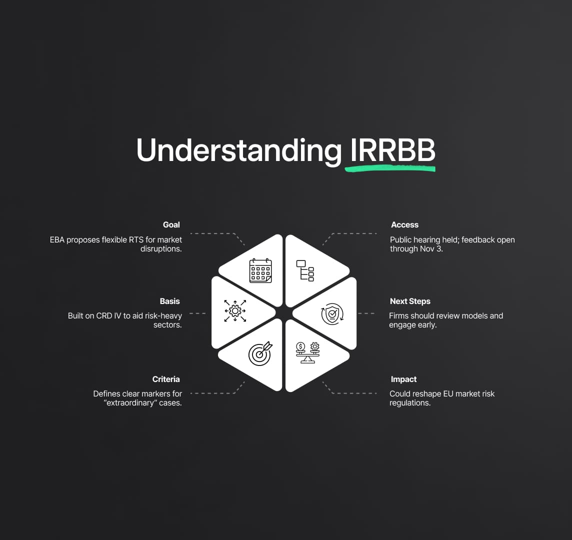
Understanding IRRBB

Interest Rate Risk in the Banking Book (IRRBB) refers to the risk to a bank’s capital and earnings arising from adverse movements in interest rates affecting its banking book positions. Unlike the trading book, which consists of assets and liabilities that are actively traded and marked-to-market, the banking book consists of assets and liabilities that are typically held until maturity. Proper management of IRRBB is crucial for the financial stability of banks and is a key component of the Basel III framework.

The IRRBB encompasses various forms of interest rate risk, including:

1. Gap Risk: Arises from the timing differences in the maturity and repricing of bank assets, liabilities, and off-balance-sheet items. This can lead to significant mismatches, affecting the bank's net interest income and the economic value of equity (EVE).
2. Basis Risk: Occurs when the interest rates of different instruments that are not perfectly correlated change in different magnitudes. This risk is particularly relevant for banks that have liabilities and assets pegged to different benchmark rates.
3. Option Risk: Involves the risk associated with embedded options in banking products, such as prepayment options in mortgages and caps/floors in floating rate loans. Changes in interest rates can alter the likelihood of these options being exercised, affecting the bank's interest income.
4. Yield Curve Risk: Arises from changes in the shape and slope of the yield curve, which can impact the valuation and interest income of bank positions across different maturities.
5. Repricing Risk: Results from the timing difference between the rate changes on assets and liabilities. For instance, if a bank's assets reprice slower than its liabilities, an interest rate hike can reduce net interest income.

The Basel Committee's IRRBB framework mandates banks to measure and manage these risks using sophisticated risk management techniques. This includes stress testing and scenario analysis to assess the impact of various interest rate movements on the bank's financial position.

---

The adjustments made by the Basel Committee in 2024 introduced several significant changes to the IRRBB standard, aimed at enhancing the precision and robustness of interest rate risk management. These adjustments include:

1. Expansion of the Calibration Time Series:
   • The time series used for calibrating interest rate shocks has been expanded to include data from December 2015 to December 2023. Previously, the calibration period extended from January 2000 to December 2015. The extended period allows for a more comprehensive analysis of interest rate movements, enhancing the robustness of shock factor determination.
2. Replacement of Global Shock Factors with Local Shock Factors:
   • The previous methodology employed global shock factors, which did not account for the unique characteristics of different currencies. The updated standard replaces these with local shock factors calculated directly for each currency. These local factors are derived from the averages of absolute changes in interest rates over a rolling six-month period, ensuring more accurate and relevant risk assessments tailored to specific currency environments.
3. Transition from 99th to 99.9th Percentile Value:
   • To enhance the conservatism of the recalibration, the percentile value used to determine shock factors has been increased from the 99th to the 99.9th percentile. This shift ensures that the shock factors remain sufficiently prudent, even in extreme interest rate scenarios, providing a higher degree of protection against potential losses.
4. Reduction in Rounding of Interest Rate Shocks:
   • Previously, interest rate shocks were rounded to the nearest 50 basis points. The new standard reduces this rounding to 25 basis points, allowing for more precise risk measurements and adjustments. This finer granularity minimizes potential distortions and better aligns with incremental changes in central banks' policy rates.

---

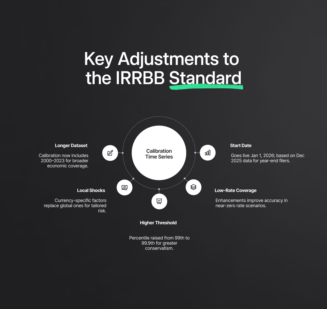
Key Adjustments to the IRRBB Standard

Expansion of the Calibration Time Series

The Basel Committee on Banking Supervision (BCBS) has significantly expanded the calibration time series for interest rate shocks, extending it from December 2015 to December 2023. The previous calibration period spanned from January 2000 to December 2015. By incorporating an additional eight years of data, the revised IRRBB standard now encompasses a broader range of economic conditions, including both periods of low and high interest rate environments. This extended time series allows for a more comprehensive analysis of historical interest rate movements, thereby enhancing the robustness and reliability of the shock factor determination process.

Replacement of Global Shock Factors with Local Shock Factors

A critical update in the IRRBB standard is the replacement of global shock factors with local shock factors. The previous methodology's reliance on global shock factors did not adequately account for the distinct characteristics and economic conditions of different currencies. The new approach calculates shock factors directly for each currency, based on the averages of absolute changes in interest rates over a rolling six-month period. This localised approach ensures that the interest rate risk assessments are more accurate and relevant, reflecting the unique characteristics, volatilities, and economic environments of individual currencies. This adjustment aligns the risk management practices with the specific conditions faced by banks operating in diverse jurisdictions.

Transition from 99th to 99.9th Percentile Value

To enhance the conservatism and robustness of the recalibration process, the BCBS has increased the percentile value used to determine shock factors from the 99th percentile to the 99.9th percentile. This significant shift ensures that the calculated shock factors are sufficiently prudent, even under extreme interest rate scenarios. By adopting the 99.9th percentile, the IRRBB standard provides a higher degree of protection against potential losses, necessitating banks to hold more capital to cover extreme interest rate changes. This increased conservatism is particularly crucial for maintaining financial stability and resilience in volatile economic conditions.

Reduction in Rounding of Interest Rate Shocks

Previously, interest rate shocks were rounded to the nearest 50 basis points. The revised IRRBB standard reduces this rounding to 25 basis points, allowing for finer granularity in the shock factor calculations. This adjustment enables more precise risk measurements and adjustments, minimizing potential distortions and better aligning with incremental changes in central bank policy rates. By reducing the rounding increment, the standard enhances the accuracy of interest rate risk assessments and improves the alignment of risk management practices with the actual movements in market interest rates.

Addressing Near-Zero Interest Rate Environments

One of the primary motivations behind these adjustments is to improve the IRRBB methodology's effectiveness during periods when interest rates are close to zero. The previous standard struggled to accurately capture interest rate changes in such environments, potentially leading to an underestimation of risks. The expanded calibration period and refined shock factor calculations are designed to ensure that the IRRBB standard remains effective under all market conditions, including low and near-zero interest rate scenarios. This enhancement ensures that banks can accurately assess and manage interest rate risks, maintaining robust financial stability even in challenging economic environments.

Implementation Timeline

The revised IRRBB standard is scheduled for implementation by January 1, 2026. Banks with a financial year ending on December 31 will need to provide the relevant disclosures in 2026, based on data as of December 31, 2025. This timeline gives banks sufficient time to update their risk management frameworks, models, and systems to comply with the new requirements. The extended implementation period ensures that banks can make the necessary operational adjustments, conduct thorough testing, and integrate the new methodologies into their risk management practices effectively. By providing ample preparation time, the BCBS aims to facilitate a smooth transition to the revised IRRBB standard, ensuring that banks are well-prepared to meet the enhanced regulatory expectations.

---

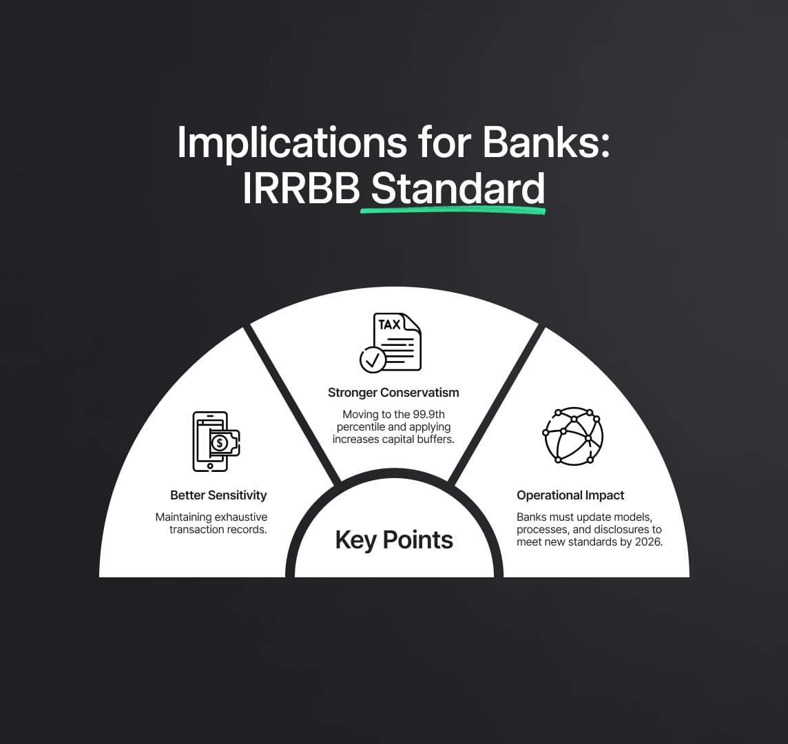
Implications for Banks: IRRBB Standard

Enhanced Risk Sensitivity and Precision

The adjustments to the Interest Rate Risk in the Banking Book (IRRBB) Standard are meticulously crafted to enhance the sensitivity and precision of interest rate risk measurements. By leveraging more localised and up-to-date data, banks can better anticipate and mitigate potential risks arising from interest rate fluctuations. The shift from global to local shock factors means that each currency's unique characteristics and economic environment are taken into account, ensuring that risk assessments are more accurate and relevant. This improvement in risk sensitivity ensures that banks' risk management frameworks are more responsive to changing economic conditions, allowing for more nuanced and effective risk mitigation strategies.

For example, the expanded calibration period from January 2000 to December 2023 includes diverse economic conditions, from periods of high inflation and interest rates to near-zero rate environments. This comprehensive dataset allows for a more robust analysis of potential interest rate movements, providing a solid foundation for determining shock factors that reflect real-world conditions.

Increased Conservatism in Risk Management

A significant aspect of the revised IRRBB standard is the shift to a 99.9th percentile value for shock factor determination, up from the previous 99th percentile. This change markedly increases the conservatism of risk measures. By adopting a higher percentile, the standard ensures that the calculated shock factors account for more extreme interest rate scenarios, providing a greater degree of protection against potential losses.

This increased conservatism translates into higher capital requirements for banks, necessitating them to hold more capital to cover potential losses from significant interest rate changes. This additional capital buffer strengthens the overall risk management framework of banks, enhancing their resilience against adverse interest rate movements. The implementation of variable caps and floors, ranging from 100 to 500 basis points depending on the scenario, further enforces this conservatism by ensuring that shock factors remain within prudent limits.

Operational Adjustments Required

To comply with the revised IRRBB standard, banks will need to undertake substantial operational adjustments. These adjustments include updating risk models to incorporate the new calibration and shock factor methodologies, revising data collection processes to ensure they align with the expanded and more detailed requirements, and enhancing disclosure practices to meet the updated reporting standards.

For instance, banks must now generate time series of daily interest rates spanning over two decades and use this data to calculate new rate change series over rolling six-month periods. This requires sophisticated data management and analytics capabilities, as well as thorough testing to ensure the accuracy and reliability of the new models. Additionally, banks will need to train their risk management teams on the updated methodologies and ensure that all relevant stakeholders are aware of the changes and their implications.

---

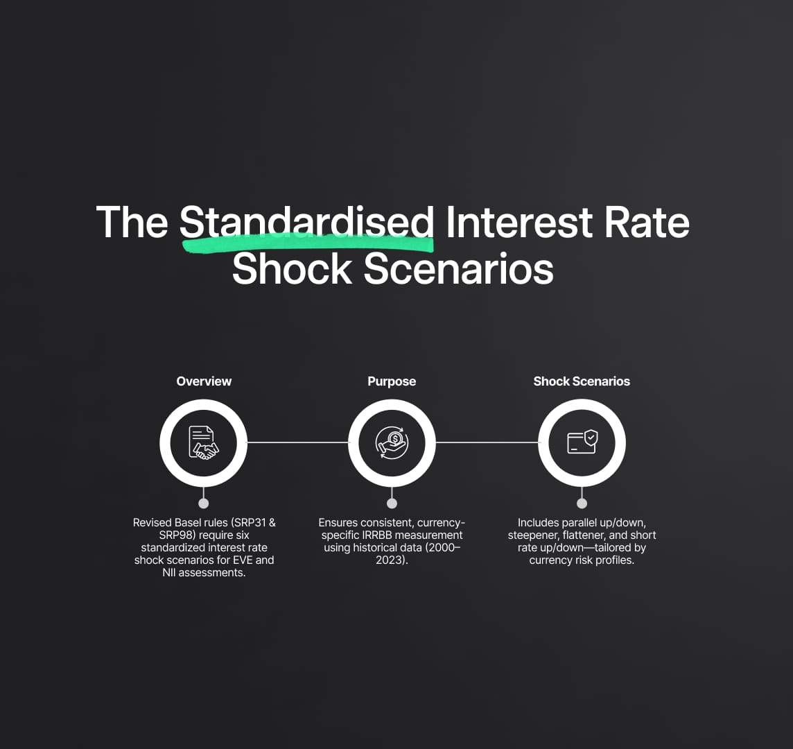
The Standardised Interest Rate Shock Scenarios

Overview

The Basel Framework revisions to chapters SRP31 and SRP98 mandate that banks apply six prescribed interest rate shock scenarios. These scenarios are designed to capture both parallel and non-parallel gap risks for the Economic Value of Equity (EVE) and two specific scenarios for Net Interest Income (NII). The detailed derivation and application of these shocks are meticulously outlined in [SRP98.56] to [SRP98.63].

Purpose and Application

The primary objective of these interest rate shock scenarios is to ensure a consistent and comprehensive approach to measuring IRRBB across banks. By applying these scenarios to IRRBB exposures in each currency where the bank holds significant positions, the standard accommodates heterogeneous economic environments across different jurisdictions. The scenarios reflect currency-specific absolute shocks, derived from historical time series data from January 2000 to December 2023, capturing the local rate environment for various maturities.

Six Interest Rate Shock Scenarios

1. Parallel Shock Up: An upward shift in interest rates across all maturities.
2. Parallel Shock Down: A downward shift in interest rates across all maturities.
3. Steepener Shock: A scenario where short rates decrease and long rates increase.
4. Flattener Shock: A scenario where short rates increase and long rates decrease.
5. Short Rates Shock Up: An upward shift in short-term interest rates.
6. Short Rates Shock Down: A downward shift in short-term interest rates.

These scenarios are crucial for accurately measuring IRRBB, as they consider both the EVE and NII impacts. Each scenario is carefully parameterized to reflect the specific economic conditions and historical rate movements of individual currencies, ensuring that the shock factors are both realistic and prudently conservative. For example, the specified sizes of interest rate shocks vary significantly by currency, with currencies like ARS and TRY experiencing higher parallel shocks (400 bps) compared to currencies like CHF and JPY (100 bps), reflecting their unique economic volatilities and conditions.

---

Specified Size of Interest Rate Shocks

The specified size of interest rate shocks in the Interest Rate Risk in the Banking Book (IRRBB) Standard is a critical aspect of the Basel Framework, tailored to reflect the unique economic conditions and historical rate movements of different currencies. This section delves into the technical details and provides a comprehensive understanding of the shock sizes, their derivation, and application.

Interest Rate Shock Sizes by Currency

The Basel Framework specifies the sizes of interest rate shocks in basis points (bps) for various currencies. These shock sizes are designed to capture the specific economic conditions and historical interest rate movements for each currency, ensuring that risk assessments are both accurate and relevant. Below is Table 2 of the Basel Framework, which details the specified shock sizes:

Currency	Parallel (bps)	Short (bps)	Long (bps)
ARS	400	500	300
AUD	300	450	300
BRL	400	500	300
CAD	200	300	300
CHF	100	150	150
CNY	275	325	200
EUR	200	300	150
GBP	275	425	200
HKD	200	300	150
IDR	400	500	300
INR	400	475	300
JPY	100	100	100
KRW	400	350	300
MXN	400	500	300
RUB	400	500	300
SAR	200	375	250
SEK	375	425	200
SGD	200	250	200
TRY	400	500	300
USD	200	300	150
ZAR	400	500	300

Recalculation of Shocks

Jurisdictions have the discretion to recalculate these shocks for their domestic currencies using data that may deviate from the initial 16-24 year period specified by the Basel Framework if it better reflects their idiosyncratic circumstances. This flexibility allows for more accurate and relevant risk management tailored to specific economic environments. For instance, if a country's economic conditions have significantly changed in recent years, recalculating the shocks using more recent data can provide a more accurate reflection of the current risk environment.

Application of Shocks

The application of these interest rate shocks involves various scenarios, each designed to test the resilience of a bank's interest rate risk management framework under different conditions. These scenarios include parallel shocks, short rate shocks, long rate shocks, and rotation shocks (steepeners and flatteners).

Instantaneous Shocks

The instantaneous shocks to the risk-free rate for parallel, short, and long scenarios for each currency are applied using specific parameterizations. These parameterizations are essential for ensuring that the shocks reflect realistic and prudent changes in interest rates across different maturities.

1. Parallel Shock for Currency c:

• A constant parallel shock up or down across all time buckets.

$$\Delta R_{\parallel,c}(t_k) = \pm \overline{R}_{\parallel,c}$$

$$\Delta S_{\parallel,c}(t_k) = \pm \overline{S}_{\parallel,c}$$

1. Short Rate Shock for Currency c:

• Shock up or down that is greatest at the shortest tenor midpoint. The shock, through the shaping scalar, diminishes towards zero at the tenor of the longest point in the term structure.

$$\Delta R_{\text{short},c}(t_k) = \pm \overline{R}_{\text{short},c} \cdot \alpha_{\text{short}}(t_k)$$

$$\alpha_{\text{short}}(t_k) = e^{-\frac{t_k}{x}}$$

$$\Delta S_{\text{short},c}(t_k) = \pm \overline{S}_{\text{short},c} \cdot \alpha_{\text{short}}(t_k) \cdot e^{-\frac{t_k}{x}}$$

1. Long Rate Shock for Currency c:

• The shock is greatest at the longest tenor midpoint and is related to the short scaling factor.

$$\Delta R_{\text{long},c}(t_k) = \pm \overline{R}_{\text{long},c} \cdot \alpha_{\text{long}}(t_k)$$

$$\alpha_{\text{long}}(t_k) = 1 - \alpha_{\text{short}}(t_k)$$

$$\Delta S_{\text{long},c}(t_k) = \pm \overline{S}_{\text{long},c} \cdot \alpha_{\text{long}}(t_k) \cdot (1 - \alpha_{\text{short}}(t_k))$$

1. Rotation Shocks for Currency c:

• Involving rotations to the term structure (steepeners and flatteners) whereby both long and short rates are shocked.

$$\Delta R_{\text{steepener},c}(t_k) = -0.65 \cdot \Delta R_{\text{short},c}(t_k) + 0.9 \cdot \Delta R_{\text{long},c}(t_k)$$

$$\Delta R_{\text{flattener},c}(t_k) = 0.8 \cdot \Delta R_{\text{short},c}(t_k) - 0.6 \cdot \Delta R_{\text{long},c}(t_k)$$

$$\Delta S_{\text{steepener},c}(t_k) = -0.65 \cdot \Delta S_{\text{short},c}(t_k) + 0.9 \cdot \Delta S_{\text{long},c}(t_k)$$

$$\Delta S_{\text{flattener},c}(t_k) = 0.8 \cdot \Delta S_{\text{short},c}(t_k) - 0.6 \cdot \Delta S_{\text{long},c}(t_k)$$

Technical Parameterisation

Short Rate Shock Example

Assume the bank uses the standardized framework with 19 time bands ($K=19$) and a time constant ($x=25$ years) for the longest tenor bucket. If the midpoint in time for bucket $k=10$ is 3.5 years, the scalar adjustment for the short shock would be:

$$\alpha_{\text{short}}(t_k) = e^{-\frac{3.5}{25}} = 0.417$$

Assume the bank uses the standardized framework with 19 time bands ($K=19$) and a time constant ($x=25$ years) for the longest tenor bucket. If the midpoint in time for bucket $k=10$ is 3.5 years, the scalar adjustment for the short shock would be:

$$\alpha_{\text{short}}(t_k) = e^{-\frac{3.5}{25}} = 0.417$$

Banks would then multiply this scalar by the short rate shock value to determine the adjustment to the yield curve at that tenor point. If the short rate shock was $\pm 100$ basis points, the increase in the yield curve at 3.5 years would be 41.7 basis points.

Steepener and Flattener Examples

For a steepener, at 3.5 years with short and long rate shocks of 100 basis points, the change in the yield curve would be:

$$-0.65 \times 100 \text{ bp} \times 0.417 + 0.9 \times 100 \text{ bp} \times (1 - 0.417) = +25.4 \text{ bp}$$

For a flattener, the corresponding change at the same point would be:

$$0.8 \times 100 \text{ bp} \times 0.417 - 0.6 \times 100 \text{ bp} \times (1 - 0.417) = -1.6 \text{ bp}$$

These examples illustrate the detailed and precise nature of the shock applications, ensuring that the IRRBB Standard effectively captures the complexities of interest rate risk across different maturities and currencies.

Interest Rate Risk in the Banking Book (IRRBB): Parameterisation Examples

In the Basel Framework, the parameterisation of interest rate shocks is crucial for accurately capturing the risk associated with changes in interest rates across different maturities. Here, we provide detailed examples of how these shocks are parameterized and applied, ensuring banks can effectively manage their Interest Rate Risk in the Banking Book (IRRBB) Standard.

Short Rate Shock

Assume a bank uses the standardized framework with 19 time bands (denoted as $K=19$) and a time constant ($t_x = 25$ years), which is the midpoint in time of the longest tenor bucket. For a specific bucket $k$, the midpoint in time ($t_k$) is given. If $k=10$ with $t_k = 3.5$ years, the scalar adjustment ($\alpha_{\text{short}}(t_k)$) for the short shock can be calculated as follows:

$$\alpha_{\text{short}}(t_k) = e^{-\frac{t_k}{x}} = e^{-\frac{3.5}{4}} = 0.417$$

Banks would then multiply this scalar by the value of the short rate shock to determine the adjustment to the yield curve at that tenor point. For instance, if the short rate shock is $\pm 100$ basis points (bps), the increase in the yield curve at $t_k = 3.5$ years would be 41.7 bps.

Steepener Shock

Assume the same point on the yield curve as above ($t_k = 3.5$ years). If the absolute value of the short rate shock is 100 bps and the absolute value of the long rate shock is also 100 bps (as for the Japanese yen), the change in the yield curve at $t_k = 3.5$ years would be the sum of the effect of the short rate shock plus the effect of the long rate shock in bps:

$$\Delta R_{\text{steepener},c}(t_k) = -0.65 \times 100 \text{ bps} \times 0.417 + 0.9 \times 100 \text{ bps} \times (1 - 0.417) = +25.4 \text{ bps}$$

Flattener Shock

The corresponding change in the yield curve for the shocks at $t_k = 3.5$ years would be:

$$\Delta R_{\text{flattener},c}(t_k) = 0.8 \times 100 \text{ bps} \times 0.417 - 0.6 \times 100 \text{ bps} \times (1 - 0.417) = -1.6 \text{ bps}$$

These calculations illustrate the detailed and precise nature of the shock applications, ensuring that the IRRBB Standard effectively captures the complexities of interest rate risk across different maturities and currencies.

---

Calculation of Interest Rate Shocks

The Basel Framework outlines a step-by-step methodology to derive interest rate shocks. This comprehensive approach ensures that the shocks are robust, accurate, and reflective of historical interest rate movements.

Step-by-Step Derivation

Step 1: Generate a 16-year time series of daily average interest rates for each currency. The average daily interest rates from January 1, 2000, to December 31, 2015, are compiled in Table 1. This table provides the average rate across all daily rates in various time buckets (3m, 6m, 1Y, 2Y, 5Y, 7Y, 10Y, 15Y, and 20Y).

Step 2: Calculate the global shock parameter based on the weighted average of the currency-specific shock parameters. The shock parameter for scenario iii is a weighted average of $\overline{r}_{i,c}$ across all currencies. The following baseline global parameters are obtained:

Scenario	Parameter	Value (%)
Parallel	$$\overline{r}_{\text{parallel}}$$	60%
Short	$$\overline{r}_{\text{short}}$$	85%
Long	$$\overline{r}_{\text{long}}$$	40%

Step 3: For each scenario iii and currency $c$, take the average of the rate changes across the corresponding time buckets in Table 1, where $N_t$ represents the number of time buckets.

$$\Delta R_{i,c}(t) = \frac{1}{N_t} \sum_{k=1}^{N_t} \Delta R_{i,c}(t)$$

Step 4: Use the 99.9th percentile value of the absolute value of $\Delta R_{i,c}(t)$ over the period from 2000 to 2023, denoted as $|\Delta R_{i,c}(t)|$, for the interest rate shock of scenario iii for currency $c$.

$$S_{i,c} = P_{99.9}(|\Delta R_{i,c}(t)|)$$

Step 5: To ensure a minimum level of prudence and a level playing field, set a floor of 100 bps and variable caps (denoted as $\overline{C}_i$) for the scenarios concerned. These caps are 500 bps for the short-term, 400 bps for the parallel, and 300 bps for the long-term interest rate shock scenario. The change in the interest rate shock for scenario iii and currency $c$ can be defined as:

$$\overline{S}_{i,c} = \max\{100, \min(S_{i,c}, \overline{C}_i)\}$$

where $\overline{C}_i = \{400, 500, 300\}$ for parallel, short, and long, respectively.

Step 6: Finally, round the values from Step 5 to the nearest multiple of 25 bps. This methodology results in the specified interest rate shocks set out in [SRP31.90].

Comprehensive Analysis

The comprehensive analysis of the parameterisation and calculation of interest rate shocks in the IRRBB Standard demonstrates the rigor and precision involved in ensuring banks can accurately assess and manage interest rate risk. By adhering to this detailed framework, banks can enhance their risk management practices, ensuring financial stability and resilience in the face of fluctuating interest rates.

---

IRRBB: Caps and Floors on Shocks

To ensure a minimum level of prudence and a level playing field in managing Interest Rate Risk in the Banking Book (IRRBB) Standard, the Basel Committee on Banking Supervision (BCBS) has implemented floors and caps on the specified interest rate shocks for different scenarios. These measures are critical in standardizing the approach across various jurisdictions and ensuring that the risk assessments are neither too conservative nor too lenient.

Specified Caps and Floors

The IRRBB framework stipulates that interest rate shock values must adhere to certain floors and caps to maintain consistency and prudence:

1. Floors: A minimum floor of 100 basis points (bps) is set for all interest rate shock scenarios. This ensures that even in low-volatility environments, banks account for a minimum level of interest rate risk.
2. Caps: Variable caps are set depending on the scenario:
   • 500 bps for short-term interest rate shocks
   • 400 bps for parallel interest rate shocks
   • 300 bps for long-term interest rate shocks

These caps prevent the shock values from becoming excessively high, which could lead to unrealistic risk assessments and overestimation of capital requirements.

Calculating Final Interest Rate Shocks

The final interest rate shocks are derived through a systematic process that involves multiple steps to ensure robustness and relevance. Here is a detailed breakdown of the final steps for shock calculation:

Step 1: Generate Historical Data Series
Create a time series of daily average interest rates ($R_{t,k}$) from January 2000 to December 2023. This data should be organized into various time buckets representing different maturities (e.g., 3 months, 6 months, 1 year, etc.).

Step 2: Calculate Rate Changes
Using the generated time series, calculate a new time series of rate changes ($\Delta R_{t,k}$) for a moving time window of 6 months (125 days). This involves computing the daily changes in interest rates within each time bucket over the specified period.

Step 3: Derive Percentile Values
Determine the 99.9th percentile of the absolute value of $\Delta R_{i,c}(t)$ over the historical period. This percentile value ($P_{99.9}$) represents the extreme movements in interest rates that the shocks are designed to capture.

Step 4: Apply Caps and Floors
For each scenario iii and currency $c$, the derived shock ($S_{i,c}$) is adjusted by applying the caps and floors:

$$\overline{S}_{i,c} = \max \{ 100, \min (S_{i,c}, \overline{C}_i) \}$$

Where $\overline{C}_i$ represents the cap specific to each scenario (500 bps for short-term, 400 bps for parallel, and 300 bps for long-term).

Step 5: Round to Nearest 25 bps
Finally, the adjusted shock values are rounded to the nearest multiple of 25 bps to maintain consistency and ease of application. This ensures the shocks are practical and straightforward for banks to implement.